Dynamic Range in Film Photography

A Complete Guide to Your Film’s Defining Characteristic

14 min read by Dmitri.
Published on December 2, 2021. Updated on October 1, 2024.

Comments

Save

7 stops of estimated dynamic range illustrated with Film Ferrania P30.

Understanding your film’s dynamic range can help improve the quality of your photography. Measured in stops or lux-seconds, your film’s DR can inform your camera settings and scene selection for optimal contrast and detail levels. Conversely, DR can guide your selection of a film stock for your scene for optimal contrast and detail in the final product. In this guide: What is dynamic range? A definition. Visualizing dynamic range — through the limitations of our eyes. The role of dynamic range in film photography. Dynamic range and film characteristic curves. How to read film characteristic curves. How to select film stock based on its dynamic range. What about exposure latitude? About film density. About image contrast. Rule of thumb. Support this blog & get premium features with GOLD memberships!

What is dynamic range? A definition.

Dynamic range is a range of intensities that a medium can record. It can be measured in decibels (for sound) but in photography, it’s measured in stops or lux-seconds.

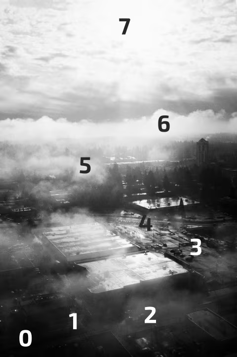
The limits of your film’s (or digital sensor’s) dynamic range can be observed in the darkest and brightest spots of photographs depicting a high-contrast scene.

Dynamic range is also sometimes referred to as tonal range. Here’s a tool for converting stops to lux-seconds and back.

Visualizing dynamic range — through the limitations of our eyes.

Have you ever looked towards the bright light and noticed that people and objects in front of it appear very dark?

Thanks to our pupillary light reflex, our irises constrict in response to bright light so that we can see better. We can adjust to changes, but can’t see well in both dark and bright light simultaneously (which is why the people/objects in front of bright light appear dark, even though you could see them well if they weren’t backlit).

This limitation of human vision (needing to adjust) is due to our eyes’ finite dynamic range. Our retinas have a limited range of light intensities they can perceive at once — beyond which everything appears either pure white or pitch black.

This range could be adjusted (shifted) with the help of the pupil that acts as an aperture (plus a few other tricks). But the range itself is relatively constant.

Photographic film has the same limitation: beyond a certain range of light intensities, it will render everything pure white or pitch black. Our cameras let us shift this range to work in brighter or darker scenes with the help of apertures, shutter speeds, and lens filters. Though shiftable, the range itself remains constant and can only be altered with your emulsion choice and the way you develop it.

View this image in HD with GOLD

Figure 1. The dynamic range of a hypothetical negative film emulsion.

The role of dynamic range in film photography.

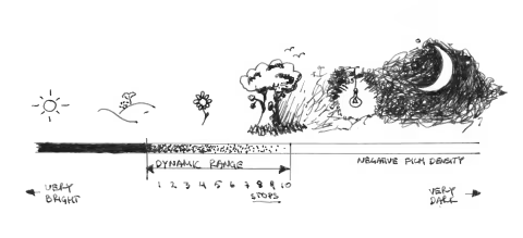
In Figure 1, above, the dynamic range of a hypothetical negative film is illustrated as a range of perceivable brightness between the sunny snow scene (second from the left) and the scene under a tree’s shade. This range is measured in stops, which is a light volume unit.

The negative film in Figure 1 can not “see” anything darker than the tree shade or brighter than white snow. The range between those brightnesses is marked to be 10 stops. Therefore, the dynamic range of that (hypothetical) film is 10 stops.

✪ Note: The shading in the “negative film density” stip in Figure 1 represents how a film negative sees the world. This is why it gets darker towards the left — when the real world gets brighter — and lighter towards the right — when the real world gets darker.

Adox CMS 20 II is an example of a high contrast narrow dynamic range film. It can capture a lot of detail, but when it comes to recording scenes with a lot of brightness variation, it easily over- and underexposes — sometimes simultaneously, like in the photograph above.

The dynamic range of your particular film will depend on the type of emulsion and how it was developed. Most colour-negative film and certain kinds of black-and-white negative film have a wide dynamic range, which can go up to 12~18 stops of light. This usually compares favourably against most digital cameras. However, some emulsions, like Adox CMS 20 II, Polaroid, and many slide film types, have much narrower dynamic ranges of about 3~5 stops.

In comparison, the human eye is often quoted to have between 10 and 14 stops of dynamic range; others quote it at 20. However, these estimates are ridden with complexities and assumptions thus, should be taken with a grain of salt.

Film’s dynamic range numbers can be found for most legacy film stocks and some new emulsions. Some manufacturers, like Kodak and Ilford, publish DR numbers with most of their emulsions. Many new films omit this information for various reasons. But it is also possible to estimate the dynamic range of your film at home.

Push-developing, a process for increasing emulsion’s effective ISO, tends to lower film’s dynamic range. Pull-developing, a process for decreasing emulsion’s effective ISO, may bump up its dynamic range. The choice of developer chemicals for black-and-white film may also affect its resulting dynamic range.

Dynamic range and film characteristic curves.

Manufacturers rarely communicate their film’s dynamic range number directly. But you can easily ascertain it from film characteristic curves graphs found in film datasheet docummentation.

Film characteristic curves — sometimes referred to as the D-Log E curve or the HD curve — plot developed film’s response (vertical y-axis) to light exposure (horizontal x-axis).

Figure 2. A hypothetical negative film characteristic curve.

Figure 2 illustrates a (simplified) hypothetical negative film characteristic curve. On its horizontal x-axis, we have increasing light intensities (exposures). On its vertical y-axis, we have the measurements of how the film responds to those light intensities (film density).

We use film density to measure how the emulsion reacts to light. The denser the film is, the more chemical compounds (grain) it has on its base that block the light from passing through.

Film characteristic curves are created by making several test exposures of the negative emulsion with increasing light intensities, which yield increasing film densities (after being developed). Those densities are then measured and plotted against the light intensities (exposures) used in the test. The more exposure (light) the negative film receives, the denser it becomes.

At some point, the negative becomes so dense that no scanner and no paper can distinguish any shades. On the other end, when the negative has virtually nothing blocking the light passing through, there are no shades to read either. Around those points are the cut-off values for the useful dynamic range of the film — beyond which a print or equalized scan will show pure white or pitch black. The distance between those two points that illustrates the dynamic range is plotted on the x-axis and measured in stops.

The steeper the curve is, the more contrasty the film is and the less dynamic range it can offer.

Slide (positive) film’s curve will slope downwards since increasing exposure will decrease the emulsion density.

Colour film will have three distinct curves plotted on the same graph, one for each channel: red, green, and blue.

Sometimes, film characteristic graphs may have multiple curves plotted for different developers and developer times. This is useful for understanding how the film may respond to being pushed, pulled, or after being soaked in a particular type of chemical bath.

How to read film characteristic curves.

The example film characteristic curves graph in Figure 2 shows no numerical values. From it, you can tell that the film is a negative-type (since the curve point upwards), that it’s black-and-white (since it has only one curve), and you may also assume that it has a wide dynamic range since the slope looks moderate. But to determine the actual dynamic range, you’ll need to read and convert some numbers.

Figure 3. A hypothetical negative film characteristic curve. Note that manufacturers list exposures in lux-seconds.

An actual film characteristic graph will have values across its x-axis (exposure) in lux-seconds (which is the output of the scientific devices that make the exposures). Lux-seconds can be converted to stops of light, which are more useful for photography.

Let’s consider another example that lists values as they appear on the manufacturers’ graphs (Figure 3). The straight portion of the graph lies somewhere between -2.8 and 0 lux-seconds, giving you 𝚫 2.8 of total lux-seconds of dynamic range.

Lux-seconds are log base 10 values which can be converted to log base 2 values used for stops of light with this formula (see full formula explanation):

log2(10^2.8) = 9.3 stops

This means that the dynamic range you have available with an example hypothetical film is 9.3 stops. Great! Now, let’s get more clarity on the above formula and how it applies to film characteristic chart values.

☝ Further reading: “Lux-Seconds, Stops, and Exposure Values Explained.”

In photography, film speed and exposure are measured in log base 2 values, meaning that each additional stop doubles the light volume. For example, EV1 is twice as much light as EV0, EV2 is four times as much as EV0, and EV3 is eight times as much as EV1.

Lux-seconds, which is a measure of one lumen (a set amount of light emitted per second) — per square metre. Lux-seconds progress in log base 10 steps. This means that 2 lux-seconds is 10 times as much light as 1 lux-second and 3 lux-seconds is 100 times as much light as 1 lux-second.

You can use this free app, your favourite scientific calculator, or approximate in your head (divide by 0.3), to make the conversion.

View this image in HD with GOLD

This scene demonstrates the power of Kodak Portra 400’s dynamic range. Here, the film captures over a dozen stops of light, ranging from reflective material highlights in full sun to deep shadows under the cars.

How to select film stock based on its dynamic range.

The physical world within your camera’s frame also has a dynamic range (often measured as contrast ratio). It can be measured in stops of light to give you an insight into how you can best capture it with your film.

A bright outdoor scene may have more than 20 stops of light variation between the deep shadows and top highlights. Meanwhile, an expertly-lit studio can have as few as 4.

To measure your scene’s dynamic range, point your spot light meter to your darkest corner and read the EV value. Then, without changing any settings, point it to the brightest highlight and read the new EV value. Then, calculate the difference between the two. The result is the dynamic range of your scene.

You can then attempt to match your film to your scene’s dynamic range. Or, if your emulsion has a narrower dynamic range than your scene, you can pick the parts of the scene you want to stay within your film’s range and which parts you will discard (and thus, appear as either pitch black or pure white).

✪ Note: Film is an imperfect medium that produces noise in the form of grain. Whenever I mention “pitch black” or “pure white” in this article, you should expect some distortion in your results, especially with colour film that often introduces colour noise in the shadows.

What about exposure latitude?

In film radiology, exposure latitude is used to describe what this article refers to as dynamic range. However, when it comes to photography, some use this term to describe an extended range of exposures film may tolerate due to its gradual falloffs near the fringes of its dynamic range.

Figure 4. A hypothetical negative film characteristic curve. On the film density axis: B-C range is the dynamic range, A-B is the toe (underexposure latitude), C-D is the shoulder (overexposure latitude).

While the useful dynamic range is defined by the straight-sloping portion of the curve, there is still some information at its ends.

In Figure 4, the bottom-left portion of the curve is called the toe; its shape implies that the film may be able to tolerate slightly less exposure than the dynamic range’s cut-off point (at the dashed line) — but not a lot and likely not well-perceived by most scanners/paper.

The top-right portion of the curve called the shoulder, implies that the film’s density continues to increase beyond the dynamic range.

The information at the toe and shoulder sections of the graph gradually becomes harder to decipher until the graph becomes horizontal — when there is 0 change in density (y-axis). However, there may still be something for your scanner or your photosensitive paper to pick up in those regions, or at least have your shadows and highlights gradually fade into nothingness instead of an abrupt cut-off. Those regions that are capable of providing some (fading) information are a part of film exposure latitude.

You may have been advised to meter for shadows when shooting negative film. It is based on the fact that negative film usually has a very good exposure latitude (gradual falloff) in the highlights. The reason for that is that the film density in the bright areas may continue to increase beyond D3.5-D4 (high/maximum measurable densities) until complete saturation. Your scanner may not be able to distinguish it very well (depending on its D-max capabilities), but the information is still there (it’s just very dark).

A good metaphor for this phenomenon is a forest at night: it’s nearly impossible to see anything without a flashlight, but we know that there are trees and grass — if only we had better eyes! By the same accord, there is likely still some visual information in a dense negative, it’s just hard to extract.

On the other hand, your scene’s shadows will be represented by the negative’s thin (least dense) parts. When there’s an insufficient amount of light for the emulsion to react to, nothing appears on the film. This “nothingness” can not gradually become “less nothing” — it’s simply blank. Because of that, the latitude of negative film for underexposure is usually negligible, and the transition into the dark regions of your print/scan (near the toe) can appear abrupt.

Metering for shadows forces your camera to favour overexposure, adding more light into the dark regions. More light means denser negatives which take better advantage of the exposure latitude.

The reverse is true for slide (positive) film, which has better exposure latitude for under-exposures.

View this image in HD with GOLD

CineStill 800T is a modern Kodak emulsion with a remarkable dynamic range. In this image, the film captures details simultaneously in the tree shadow and within the sunburst without any banding or extreme distortions. If you subscribe to the film latitude definition in this article, you’ll notice plenty of it in this emulsion’s ability to gradually fade regions out of its dynamic range into pure whites and pitch blacks.

About film density.

Like an inkjet print, exposed film is a collection of black dots. There is no greyscale, no gradients — darker shades are represented by more densely packed activated silver halide crystals, lighter shades — more sparsely packed “dots” (grain). Those “dots” are arranged in an incredibly complex pattern that follows the chemical and physical structure of the emulsion as it reacts to infinitely diverse travel paths of photons.

When we look at or scan film, we see gradients when there are none. This is because a single scanned pixel (or a dot in our vision) contains a variable number of grains, more of which will look like a darker pixel/dot and less — lighter.

You can observe this effect by looking at the shading in Figures 1, 2, and 4, which represents film density. I drew dots, which are always 100% black, but their density can appear as shades of grey if you stand back far enough.

Film density is measured using densitometers with D-units that range from 0 to 4, where 0 is air and 4 is an opaque medium. Note how the density of the film in the characteristic curves never starts at zero: this is because the translucent emulsion base has some opacity to it.

The resolution of the film density is limited by the device that measures it (i.e., your film scanner or a densitometer) and the noise that film grain introduces into the mix. An infinitely small grain with an infinitely precise measuring device can theoretically offer an infinite density resolution (which we subsequently perceive as shades of grey or colour). But, of course, that is never the case.

In the digital world, each pixel/point has an actual shade, which is represented using a finite value, typically from 0 to 255 (for 8-bit/channel). A single pixel can paint exactly 256 different shades of grey.

For colour, both film and digital medium employ channels, which can be thought of as three distinct greyscale images tinted in either red, green, or blue. When combined, they create a full-colour picture.

☝ Further reading: “All you need to know about Densitometers” — Firstcall-Photographic. This article should be a good starting point for understanding the film density values on the y-axis of the film characteristic graphs and the tools used to produce them.

View this image in HD with GOLD

Adox CMS 20 II’s remarkably narrow dynamic range is used in this photograph, taken during a foggy afternoon, to distinguish slight variations in shading that would otherwise be invisible or distorted on wide dynamic range emulsions.

About image contrast.

The dynamic range of film directly affects its contrast. A narrower dynamic range means higher contrast and vice-versa.

It’s possible to increase or decrease image contrast without changing its dynamic range. This can be done digitally after scanning the film. However, strong changes in contrast can erase detail and introduce banding to images. You may also choose to alter your photograph’s contrast in development or while printing in a darkroom — doing so will also typically erase detail and introduce analogue distortions.

The safest method for retaining maximum detail from film is usually shooting it and developing normally (which would typically yield the finest grain — as opposed to using experimental developers or push/pull processing).

Out of the box, low-ISO films will often render higher-contrast images with finer grain, whereas high-ISO films will typically produce lower-contrast photos.

Rule of thumb.

To tie everything above into a compressed guideline: lower-ISO films may work best with low-contrast scenes (such as foggy days and shady areas), whereas higher-ISO films will show more detail in shadows and highlights in bright light. Film’s listed dynamic range can inform you even better with numbers like 3 stops, meaning high contrast with a high chance of detail loss in shadows/highlights and 12 to 18 stops being able to capture light as well or even better than our eyes.

Sign in to continue reading (free).

Your free Analog.Cafe account gives you access to web apps, downloads, exclusive content, and more!

Continue with Google

By creating and using an account you agree to Terms, Use, and Privacy Policies.
Sign In Help

Techniques like dodging and burning shows us that at least many black and white films have dynamic ranges bigger than what human eye can register. It’s often shock to many people to see how you can “recover” details from “underexposed” or “overexposed” by adjusting time of exposure of print paper in darkroom or by adjusting level of backlight during scanning. And the bigger film format is used the dynamic range only increases.

What is dynamic range? A definition.

Visualizing dynamic range — through the limitations of our eyes.

The role of dynamic range in film photography.

About this article:

Dmitri